A/B Testing, Part 1: Random Segmentation
A/B Testing Series
- Random Sampling
- Statistical Significance
- Fisher's Exact Test
- Counterfactuals and Causal Reasoning
- Statistical Power
- Confidence Intervals
Introduction
Often times we want to influence the behavior of others through our own actions. That sounds manipulative, but here are some innocent examples:
- Designing a better resume to get more job leads.
- Choosing a profile picture to get more likes.
- Tweaking a recipe to brew better beer.
When considering our options, the methods of statistics allow us to estimate which option is best and can even provide an estimate of how much better it is relative to the alternatives.
By far the most common application of these principles is in the tech world, so for the sake of this discussion, let’s talk about email subject lines and open rates. If we are designing an email marketing campaign, we want to choose a catchy subject line that gets the most people to open the email. We might have several candidates we want to test, but for simplicity, let’s suppose there are only two subject lines, which we will refer to as $A$ and $B$.
Let’s say there are a thousand recipients ($n=1000$) in our audience. Suppose we decide we like subject line $A$ the best and send it to everyone, and one hundred people open it, so the open rate is $10\%$. We’ll call this number $p_A$. This number represents an observational fact! Later in our discussion, some numbers will represent estimates or probabilities, and it is important to recognize the distinction. Sometimes people will use phrases like, “the probability that someone will open the email,” but that isn’t right. A person either opens the email, or they don’t. Probability has nothing to do with it.
We can only speculate about what would have happened had we gone with the other subject line. Since we are supposing quite a bit, let’s say we have a magical crystal ball that allows us to see into a parallel reality where we had used subject line $B$, and in that reality, one hundred and twenty people opened the email, for an open rate of $12\%$. We’ll call this number $p_B$. This number is also an observational fact—we just needed a crystal ball to observe it. Even though it is speculation, it still has nothing to do with probability. It is not the probability that someone would open the email had we used subject line B. Had we done that, the person still either would have opened it, or they wouldn’t have.
Knowing both $p_A$ and $p_B$ (thanks to our crystal ball), it is easy to determine that the second subject line is better, resulting in $20\%$ more opens. Unfortunately, we don’t really have a magical crystal ball. Nonetheless, we would like to find a way of determining which subject line is better, and by how much.
When I talk to people about A/B testing, this crystal ball stuff seems to be the most confusing. (Or maybe they just stop paying attention before I get to probability, which I would expect to be the more confusing part.) Either way, it’s worth spending just a little more time on it.
In other talks, I have used analogies referencing Back to the Future and Groundhog’s Day, but perhaps the simplest way to grasp it is to consider that every action has consequences. We don’t need to guess what the consequences of any action are, we simply take that action, and witness the consequences. But we can only witness the consequences of the choice we made, not the choices we didn’t make. We can make a different choice “next time,” but there is no guarantee that what happens next time, is what would have happened this time. That doesn’t change the fact that something would have happened. It just isn’t obvious how to figure out what that would be. Though magic has failed us, science will not!
It is intuitively obvious we need to actually try both options in order to determine which is better. For a recurring email campaign, we might try subject line $A$ on Monday and subject line $B$ on Tuesday and compare the open rates. If we assume the people receiving the email on Monday behave the same way as the people who receive the email on Tuesday, this might make sense. The problem is, this is a ridiculous assumption. No two people ever behave exactly the same way, so the idea that a large group of people would behave the same way as some other large group of people is ludicrous.
And yet, in my experience important metrics do tend to exhibit some consistency over time. If the open rate is 10% on Monday, it would be surprising if it were exactly 10% on Tuesday, but it would also be surprising if it increased to 90%. On the one hand, because human behavior is so complicated, exact consistency just isn’t plausible. On the other hand, the people receiving the email on Tuesday probably have a lot in common with the people receiving the email on Monday. If nothing else, they all belong to the “target audience”, e.g. people who shopped at a particular store, or who expressed interest in a specific product. So we would expect similar people to have similar reactions to the same subject line – just not identical reactions.
Simply plotting a metric over an interval—during which our own behavior does not change—provides the best estimate of how much “natural” variation to expect. If we try subject line $A$ on Monday, and $B$ on Tuesday, we have to ask if the observed difference in open rates is in line with the normal daily variation. If there is only a small improvement from Monday to Tuesday, we cannot determine whether the difference is due to the changed subject line, or due to the daily variation. Even if there is a large change, much larger than usual, we are left wondering whether there was some other impetus that occurred, coincidentally, at the same time. In short, if $B$ is only slightly better than $A$, we won’t even notice, and if $B$ is significantly better, we may misattribute the improvement to some other factor. There is a better way!
Random Sampling
We saw how useful a crystal ball would be, if one existed. We now introduce a device, called a random sample, that allows us to predict the consequences of the choices we didn’t make. The cost of employing such a device is enduring a modest amount of statistics. Ye be warned.
Starting from a countable set of objects called the population, a sample is a finite collection of objects drawn from the population with or without replacement. For example, given the population {cat, dog, mouse, hamster}, the following is an exhaustive list of all samples of size two, drawn with replacement:
- {cat, cat}, {cat, dog}, {cat, mouse}, {cat, hamster},
- {dog, dog}, {dog, mouse}, {dog, hamster},
- {mouse, mouse}, {mouse, hamster},
- {hamster, hamster}
We consider the sample {cat, dog} to be the same as the sample {dog, cat} (though in different applications, this may not always be the case). If we were sampling without replacement, each object in the population could appear at most once in a sample. When there are $n$ objects in the population, there are ${n + k - 1 \choose k} = \frac{(n+k-1)!}{k! (n-1)!}$ possible samples of size $k$ drawn with replacement, and ${n \choose k} = \frac{n!}{k! (n-k)!}$ possible samples drawn without replacement.1 Any mechanism for selecting one of these samples—in an unpredictable way—is called a random sampling method, and the result of such a selection strategy is called a random sample. We might envision writing them all down on slips of paper and selecting one of them out of a hat, or throwing a dart at a wall, although these turn out to be not very good methods.
Sometimes the size of the sample is selected in advance; sometimes it is the incidental outcome of the sampling method itself. For now, we will restrict ourselves to sampling methods where the sample size is fixed by design. We will also assume that the sampling method is such that all samples are equally likely to be selected.
Once we have introduced the concept of randomness, it becomes possible to ask questions about how likely certain things are to happen. For example, revisiting our exhaustive list of samples of animals, we see that four out of ten samples contain a cat, so we say the probability of a random sample containing a cat is $40\%$. This probability corresponds to the frequentist interpretation, in which probabilities represent the fraction of all possibilities that satisfy some criterion. (When the population is infinite, it becomes conceptually more challenging to interpret these probabilities. For our purposes, the population will always be finite, but typically having many more than ten elements.)
The Law of Large Numbers
Let’s return to our thousand email recipients. This is our population. Suppose we send subject line $A$ to everyone; recall from our prior discussion that one hundred people opened the email. We say that the population open rate is $10\%$. We again emphasize this represents an observational fact, not a probability. Let’s consider a random sample of size five hundred, drawn without replacement from the population. How many people in the sample do we expect to open the email? It is certainly possible that all one hundred email-openers wound up in our sample, so the sample open rate could be as high as $20\%$. It could also be as low as $0\%$, if by chance no email-openers wound up in our sample. Intuitively, these seem unlikely outcomes, and if we were to make a list of all ${n \choose k} \approx 2.7 \times 10^{299}$ possible samples, we would see that about $8.6 \times 10^{266}$ of them contained one hundred email openers. In other words, about one in $3 \times 10^{32}$ samples has one hundred email openers. We are about as likely to win the lottery four times in a row as we are to draw such a sample.
On the other hand, about $8\%$ of samples contain exactly fifty email openers. For these samples, the sample open rate is exactly equal to the population open rate, $10\%$. Note the two interpretations of percentages: $8\%$ represents a fraction of all possible samples; $10\%$ represents the sample open rate for these particular samples. We interpret the former as a (frequentist) probability; the latter as observational facts having nothing to do with probability.
While it would hardly be remarkable to draw a sample whose open rate exactly matched the population, it also isn’t very likely. In fact, for $92\%$ of samples, the sample open rate is not equal to the population open rate. If we choose a sample at random, the sample open rate will most likely not equal that of the population. On the other hand, most samples do not deviate too far from the population open rate: about $54\%$ of samples have a sample open rate between $9.4\%$ and $10.6\%$, and about $95\%$ of samples have a sample open rate between $8.2\%$ and $11.8\%$.
These numbers are specific to the case of 1000 email recipients, 100 email openers, and a sample size of 500. The cumulative distribution function of the hypergeometric distribution allows us to compute the numbers quoted above, as well as for situations with arbitrary parameters. With the numbers above, we saw that $95\%$ of samples had a sample open rate that was within $\pm 1.8\%$ of the population open rate. We will call this number the plausible error. (This general concept comes in many forms; here we mean that number $\epsilon$ such that $\operatorname{P} [| s - p| \leq \epsilon ] \geq 95\%$, where $s$ is the sample open rate, and $p$ is the population open rate. The probabilistic notation should be interpreted as the fraction of all samples satisfying $|s - p| \leq \epsilon$.)
Figure 1 shows how the plausible error depends on the size of the sample. For this figure, the sample size is always half of the population, and the population open rate is always $10\%$. We see that the plausible error decreases to zero as the population and sample sizes get larger. In other words, as the sample size gets larger, it becomes increasingly unlikely that the sample open rate deviates very far from the population open rate. This is an illustration of the Law of Large Numbers.
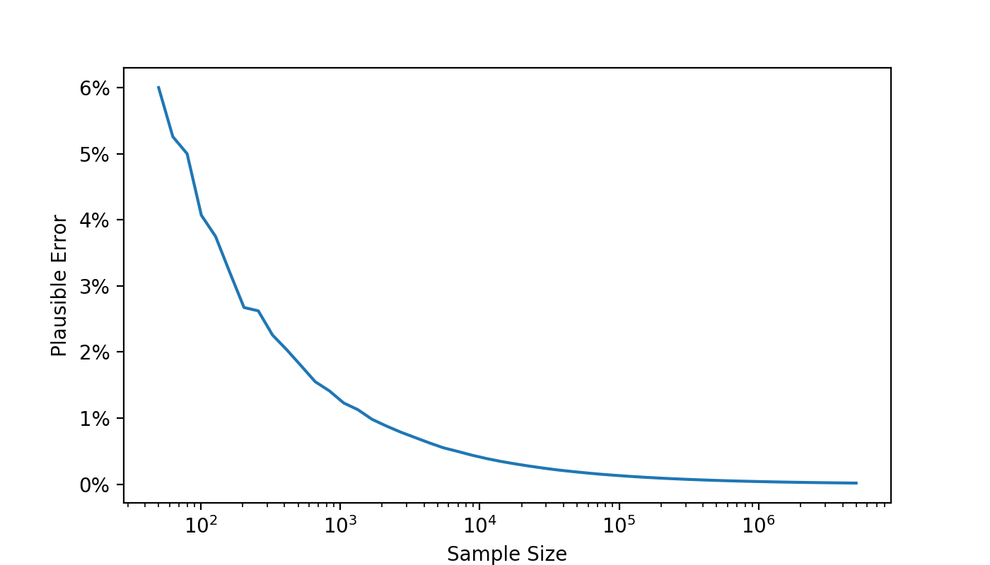
Plausible Error
Random Segmentation and Causal Inference
The Law of Large Numbers states that for a large enough sample size, we can get an arbitrarily good estimate of population behavior based on sample behavior. In terms of the example we have been using: the open rate of a sample is approximately equal to the population open rate, for the overwhelming majority of samples we might possibly draw. The larger the sample size, the closer the approximation.
Thus if we divide the population in two segments, and send subject line A to the first segment, the open rate in that sample is a good approximation to what the population open rate would have been, had we sent subject line A to the entire population. Similarly, if we send subject line B to the second segment, the open rate in that sample is a good approximation to what the population open rate would have been, had we sent subject line B to the entire population. The process of randomly dividing a population into two or more groups and providing different experiences to each group as a way of comparing the consequences of different choices is called A/B testing.
This only works assuming negligible interaction between the segments. If someone in the first segment calls their friend in the second segment telling them about the email subject line they got, it may affect their friend’s decision of whether to open the email. In this context, it seems ridiculous, but in social networks, this phenomenon must be addressed.2
With a crystal ball, we could magically determine the consequences of the choice we didn’t make. Random sampling is almost as good; instead of being able to determine exactly what would have happened in a parallel reality, we are forced to accept an approximation. But when the sample size is large, it is a very good approximation, and can form the basis of legitimate conclusions about which choice is better.
Because we are effectively pursuing both options simultaneously, it rules out the possibility of any other factors influencing the results. Even if marketing activities have lead to a dramatic increase in open rates on the same day that we are conducting the experiment, that marketing impact applies equally to both segments. Thus, random segmentation isolates the impact of the choice under consideration from that of any other factors. In this sense, random segmentation allows for truly causal inference.
Sampling a Stream
When we have a fixed group of people that we want to divide, the above method works well. Often times, we need to segment a population, but we don’t actually know how big the population is in advance. For example, we might want to A/B test a welcome email to be sent as soon as a person signs up. Rather than choosing a sample of a given size, all at once, we can assign each individual to a segment, one by one. We just flip a coin each time someone signs up, and use the outcome to decide which segment to assign the person. Equivalently, choose a uniform random number between 0 and 1, and assign the user to the first group if it is less than 0.5, otherwise to the second group. It is easy to see how to generalize this concept to uneven group sizes, like if we wanted to send email A to $90\%$ of users.
This approach is often preferable to the random sampling approach, even when the population is fixed in advance. Many programming languages do not support random sampling from a population, but virtually all programming languages can generate uniform random numbers.
Of course, flipping a coin for each user will not divide the population exactly in half. If we are segmenting ten users in this way, it’s entirely plausible we might get seven heads, resulting in only three recipients of the second variant. The Law of Large Numbers assures us that if the total number of people to be segmented is large, the split will approximately match the desired result.
If we use this approach, we should use the binomial distribution to analyze the results, instead of the hypergeometric. Often, tools will use an approximation based on the normal distribution for either situation. We will consider the different options in a later post.
Pseudorandom Sampling
Unless you are using a quantum device, whatever sampling method you are using is not really random. But the pseudorandom numbers that computers generate can be just as effective. All we really need is for the segmentation of each person to be independent of any of their characteristics. If we have some unique identifier for the person, we can choose from a variety of hashing function to divide people into groups. This deserves a post of its own.3