Sensitivity Analysis for Matched Pairs

- 1 Introduction
- 2 Intuition
- 3 Example #1: TV Measurement
- 4 Example #2: Survey-Based Measurement
- 5 Coda
- 6 Stochastically Increasing Vectors
- 7 Test Statistics for Matched Pairs
- 8 Strong Ignorability and The Distribution of Treatment Assignments
- 9 The Differences in Treatment Assignments is Stochastically Increasing in the Difference in Unobserved Covariates
- 10 Extreme Configurations
- 11 Sensitivity Analysis with Large Sample Sizes
- 12 Sensitivity Intervals and Hybrid Sensitivity/Confidence Intervals
- 13 The Capacity of an Observational Study
- 14 Two-Sided Tests
- 15 Summary
- 16 References
1 Introduction
About a year and a half ago, I read, “Observation & Experiment” (Rosenbaum 2019). Although it doesn’t go into much mathematical detail, it’s a treasure trove of ideas relevant both to randomized experiments and observational studies.
The book discusses uncertainty in an observational study resulting from unobserved confounding factors. I like to say data science is about managing uncertainty. Uncertainty comes from many sources, like random sampling from a population, or model drift (training a model on past data but applying it to future observations). Quantifying uncertainty is the first step towards managing it.
In an observational study, factors correlated with both the treatment and outcome (confounders) can distort the observed relationship. These factors may lead us to conclude a treatment is beneficial, when in fact it is harmful, a phenomenon known as Simpson’s paradox. We may adjust for observed confounders to remove overt biases, but we cannot adjust for unobserved confounders.
Outside of a controlled, randomized experiment, unobserved confounders are always possible, introducing uncertainty into the conclusions of any observational study. Rosenbaum has developed an approach for quantifying the sensitivity of study conclusions to these hidden biases. Rosenbaum developed the approach over several key papers. I set myself the challenge to work through each paper. In this post, I will review the 1987 paper, “Sensitivity Analysis for Certain Permutation Inferences in Matched Observational Studies” (Rosenbaum 1987).
2 Intuition
The paper discusses studies involving pairs of units. Within each pair, one unit experiences the treatment condition and the other unit experiences the control condition. In subsequent papers, Rosenbaum extended the method to matching with multiple controls, and unmatched studies. Here we focus only on matched pairs.
In a randomized experiment, we decide on some appropriate test statistic, \( T, \) having a known distribution under the null hypothesis. Using that null distribution, we compute the probability of the test statistic exceeding its observed value. The resulting p-value quantifies the amount of bad luck required to explain the observed result (Rosenbaum 2015, sec. 1.2), by reference to a \( U(0, 1) \) distribution.
In an experiment with a p-value of 0.01, the observed association could be spurious, but only through quite a bit of bad luck. A spurious association in this case would be like sampling from a \( U(0, 1) \) distribution and getting a result less than 0.01. The p-value does not tell us whether bad luck occurred; it tells us how much bad luck would have been involved were the association spurious. A p-value facilitates discussion about the strength of evidence in an experiment by expressing it in terms of bad luck.
Test statistics aren’t useful only for calculating p-values. We may calculate a point estimate using the Hodges-Lehmann trick (Hodges and Lehmann 1963). We may compute a confidence interval on the treatment effect by inverting the test (Casella and Berger 2002). Inference hinges on a known null distribution for the test statistic.
In an observational study, we do not know the null distribution of the test statistic as it may depend on unobserved factors. A sensitivity analysis quantifies how strongly these factors would have to skew the treatment selection mechanism to explain the observed result. The analysis does not tell us whether such skew was present (just as a p-value does not tell us whether bad luck occurred). Rather, the analysis facilitates discussion about the strength of evidence by expressing it in terms of skew.
A sensitivity analysis determines two distributions bounding the true, unknown distribution of the test statistic. These bounding distributions allow us to calculate bounds on the p-value, point estimate, and confidence interval.
The bounds on the p-value lead to a strength-of-evidence metric, \( \Gamma^\star, \) appropriate for observational studies. This metric combines the notions of bad luck and treatment selection skew discussed above. Reporting \( \Gamma^\star \) does not tell us whether such bad luck occurred, or whether such skew was present. Rather, it facilitates a discussion about strength of evidence.
A sensitivity interval bounds the point estimate we would have calculated based on \( T. \) Just as a confidence interval quantifies the uncertainty on the effect size that comes from probabilistic treatment assignment, a sensitivity interval reflects the uncertainty that comes from the possible impact of unobserved confounders. These sources of uncertainty, probabilistic assignment and unobserved confounders, may be combined into a joint sensitivity/confidence interval.
3 Example #1: TV Measurement
Rosenbaum includes a few examples in his paper, but I found it helpful to invent my own examples. Both relate to measuring the impact of TV advertising. TV ad measurement is challenging for several reasons: we can’t run user-level randomized holdouts; we don’t have a list of people who saw the ad; the impact of the ad may not be instantaneous but rather cumulative over long time periods.
Still, if TV ads were effective, and if we showed ads in some years but not others, we would expect to see more purchases in the years with ads than without. While we could randomly assign the TV ad budget over many years, no business would ever go along with it. Instead we might try to exploit haphazard variation in the budget, perhaps as the economic environment changes, or as different leaders execute different marketing strategies.
We assume we have several years of sales data. In some years, marketing spend on TV ads was high, and in other years it was low. We will interpret “low” as non-existent, and we will treat all “high” years as having the same spend. (A more detailed model would take the spend levels into consideration.) We also assume years have been paired in a sensible way, accounting for economic and other factors.
The table below presents ten years of 100% made up sales data.
| Pair | Control | Treated | Treated Minus Control |
|---|---|---|---|
| 1 | 1,000 | 1,100 | 100 |
| 2 | 500 | 490 | -10 |
| 3 | 1,500 | 1,700 | 200 |
| 4 | 700 | 720 | 20 |
| 5 | 400 | 370 | -30 |
The average difference in sales, treatment minus control, is 56. If marketing had been assigned at random each year, and if we ignored the uncertainty associated with such small samples, we would conclude that TV advertising led to an average of 56 additional sales per year.
>>> d = [100, -10, 200, 20, -30]
>>> def t(d):
...     return sum(d) / len(d)
>>> print("T_obs = {0:.0f}".format(t(d)))
T_obs = 56
There are \( 2^5 = 32 \) patterns of treatment selection within 5 pairs. A one-sided p-value is the fraction of these 32 possibilities leading to a mean treatment-minus-control statistic of at least 56. There are 6 such patterns, including the pattern that actually occurred. The one-sided p-value is thus 6/32 = 0.1875. This would not be considered significant at the conventional level of 0.05. With such small sample sizes, that’s unsurprising.
>>> import itertools
>>> def prob(v):
...     """Calculate the probability that V=v."""
...     return 1 / (2 ** len(v))

>>> def pval(d, tau0=0.0):
...     """Calculate the probability that t(d, V) >= t_obs."""
...     p = 0
...     S = len(d)
...     t_obs = t([ds - tau0 for ds in d])
...     for v in itertools.product([-1, 1], repeat=S):
...         if t([vs * (ds - tau0) for vs, ds in zip(v, d)]) >= t_obs:
...             p += prob(v)
...     return p
>>> print("p = {0:.04f}".format(pval(d)))
p = 0.1875
A one-sided 95% confidence interval on a constant additive effect is \( \geq -30. \) That is, although the result is not statistically significant, and we therefore can’t prove the TV ads increased sales, we can rule out the possibility that TV ads decreased sales by more than 30 sales per year. (Since these are made up numbers, I could have come up with an example that was statistically significant, but I elected to use an example I think is more realistic.)
>>> for tau0 in (-30, -31):
...     print("p = {0:.04f} (against tau = {1:.0f})".format(
...         pval(d, tau0), tau0
...     ))
p = 0.0625 (against tau = -30)
p = 0.0312 (against tau = -31)
These numbers—the point estimate, the p-value, and the confidence interval—are only valid if matching years into pairs adjusts for all factors relevant to the choice to advertise or not advertise. If so, two years in a pair are interchangeable: no differences between them are relevant to the decision to advertise. From that symmetry principle, each year is equally likely to have used advertising.
Important differences may remain, perhaps unobserved differences. In that case, the two years are not interchangeable: one year had characteristics encouraging the business to advertise in that year rather than the other.
A sensitivity analysis explores the spectrum of deviations from complete interchangeability. At one extreme, we have the ideal of the randomized experiment, where each year in a pair is equally likely to have used advertising. At the other, we have selection on outcomes: with perfect foresight, we advertise in the years where advertising is most beneficial, and we don’t advertise in years where advertising would be ineffective.
The reality is likely somewhere in between. We quantify locations along this spectrum with an odds ratio. If the two years in a pair are interchangeable, there is even odds (odds ratio of 1) as to which year the business advertised. In the perfect foresight, selection on outcomes scenario, the odds ratio is infinite.
Figure 1 shows the uncertainty in the point estimate along two dimensions. We plot the deviation from random assignment along the x-axis in terms of the odds ratio, \( \Gamma. \) For each value along this spectrum, we portray the impact this deviation may have on the point estimate as a sensitivity interval. The dashed line in the middle shows the point estimate we reported above: 56 incremental sales per year. The solid lines show that as we deviate farther from perfect interchangeability within pairs, there is more uncertainty about the point estimate we would calculate had we observed all relevant covariates. The solid lines asymptotically approach the outer dashed lines.
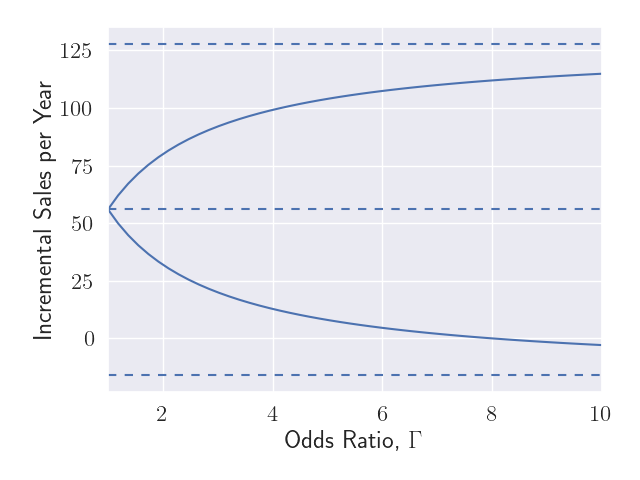
Figure 1: Sensitivity Interval
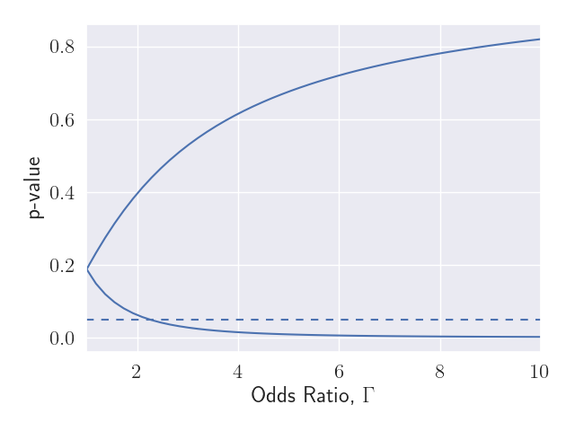
Figure 2: P-Value Interval
Figure 2 shows the range of p-values we might calculate, if we observed all relevant factors. A statistically significant result (\( p < 0.05 \)) would only occur if (i) the unobserved factors skewed the treatment selection quite a bit (\( \Gamma > 2.25 \)) and (ii) these unobserved factors were sufficiently correlated with sales. A value of \( \Gamma = 2.25 \) corresponds to advertising being 2.25 times more likely to have occurred in one year in the pair vs the other. We would have to think about what factors might lead to such a skew and try to add them to our analysis.
Based on Figure 2, we can report \( \Gamma^\star = 1 / 2.25 = 0.44 \) as a strength of evidence metric for this study. Larger values of \( \Gamma^\star \) represent stronger evidence. A value of \( \Gamma^\star < 1 \) indicates that even had we adjusted for all relevant factors, the study would still not represent strong evidence of an effect. And since there may be other factors not included in the analysis, the evidence is even weaker than this.
The capacity of this study is \( \Gamma = 1.2. \) If the confounding is worse than this, the study is completely uninformative in the sense that the uncertainty region includes all patterns of treatment effects. One implication is that the combined sensitivity/confidence region on the average treatment effect is unbounded in both directions. \( \Gamma > 1.2 \) indicates there is at least one pair having one year more likely to have used advertising than the other, with an odds ratio of \( > 1.2. \) We would have to be very confident in our adjustments to rule out that possibility.
4 Example #2: Survey-Based Measurement
Suppose we fielded surveys with questions about exposure to TV advertising (“do you recall seeing a TV ad for <brand>?”) and perception of the brand (“how would you rate your perception of <brand>?”). Supplemental questions would ask about likely confounding factors that might explain why a person would or would not have seen the TV ad.
Suppose we get a few thousand responses and use the supplemental questions to create pairs. Within each pair, one person recalls seeing a TV ad and the other does not. Otherwise, the two people within a pair are as similar as possible in terms of responses to the supplemental questions.
We can group the pairs into three categories:
- concordant pairs where the two people have the same brand perception;
- discordant pairs where the person who recalled seeing the ad had better brand perception than the person who didn’t; and
- discordant pairs where the person who recalled seeing the ad had worse brand perception.
If the matching adjusted for all relevant factors, and TV advertising improved brand perception, we would expect more pairs in category 2 than in category 3. This is the basis for McNemar’s test. (This test completely ignores the concordant pairs.)
Suppose there were 2,700 pairs in category 2 and 300 pairs in category 3. If respondents had been randomly assigned to receive or not receive marketing, the number of pairs in category 2 would have a Binomial distribution with probability of success 0.5 and 3,000 trials. A p-value against the null hypothesis of no effect would be vanishingly small.
>>> import scipy.stats as stats
>>> print("p = {0:.03g}".format(
...     stats.binom(3_000, 0.5).sf(2_700)
>>> ))
p = 0
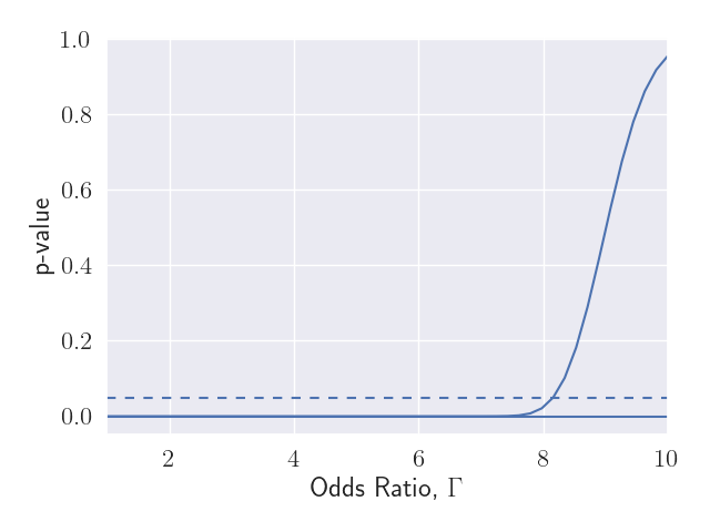
Figure 3: P-Value Interval
Figure 3 shows the range in p-values as we consider larger departures from the ideal of a randomized experiment. The dashed line shows the significance threshold, 0.05. We see that when \( \Gamma > 8, \) the upper bound on the p-value exceeds this threshold, so the sensitivity of the study is around \( \Gamma^\star = 8. \)
This study is much less sensitive to hidden biases than the previous example, but note also that the pattern of brand perception was remarkably consistent. In 90% of the discordant pairs, it was the person who remembered seeing the ad who had the better brand perception (the treated person). It is unusual to see such consistent results.
A more realistic example might have 2,000 pairs where the treated person had the better brand perception out of 3,000 discordant pairs total. The p-value is still vanishingly small, but now \( \Gamma^\star = 1.878. \) A larger sample size achieves only a small improvement: with 20,000 pairs out of 30,000, \( \Gamma^\star = 1.96. \) A 10x increase in sample size achieved only a modest improvement in sensitivity.
In a randomized experiment, a larger sample size improves statistical power by reducing variance. The uncertainty in an observational study is not just about variance, but primarily about bias. Larger sample sizes do not decrease bias. On the other hand, larger effect sizes do tend to reduce sensitivity to hidden biases.
5 Coda
Readers content with intuition should stop reading now. Other readers who would like to do their own sensitivity analyses, but who do not feel the need to understand the derivations, should read the rest of this section. The derivations making up the rest of this post are fairly sophisticated, but the final formulae are comparatively simple.
The sensitivity of an observational study, \( \Gamma^\star, \) is defined immediately following Equation (\ref{eqn:gamma_star}). The sensitivity is a strength of evidence metric appropriate for an observational study.
The capacity of an observational study is defined in Equation (\ref{eqn:capacity}). The capacity is a simple function of the sample size and the desired Type-I error rate, and puts a limit on what may be learned from an observational study. Any observational study becomes completely uninformative if there are enough unobserved confounders.
The bounds on a sensitivity interval are given by (\ref{eqn:sensitivity_interval}). A large sample approximation to the upper bound on the p-value is given by Equation (\ref{eqn:asymptotic}). This approximation is useful also for calculated combined sensitivity/confidence intervals.
6 Stochastically Increasing Vectors
The key result in (Rosenbaum 1987) hinges on a lemma from (Ahmed, Leon, and Proschan 1981) regarding stochastically increasing vectors. Suppose we have two vector-valued random variables, \( X \) and \( Y \). Each variable has some pre-order associated with it. A pre-order on a set \( \mathcal{X} \) is a relation \( \preceq \) satisfying (i) \( x \preceq x \) for all \( x \in \mathcal{X} \) and (ii) \( x \preceq y \) and \( y \preceq z \) implies \( x \preceq z \) for all \( x, y, z \in \mathcal{X}. \) The pre-orders for \( X \) and \( Y \) are potentially different: call the pre-order associated with \( X, \, \preceq^\prime, \) and with \( Y, \, \preceq^\ast. \)
A function, \( f : \mathcal{X} \to \mathbb{R} \) is said to be increasing with respect to \( \preceq \) if \( x \preceq y \) implies \( f(x) \leq f(y) \) for all \( x, y \in \mathcal{X}. \) (Ahmed, Leon, and Proschan 1981) offers the following definition: a random vector \( Y \) is said to be stochastically increasing in the random vector \( X \) with respect to \( \preceq^\prime \) if \( h_f(x) := E[f(Y) \, | \, X = x] \) is increasing in \( x \) (with respect to \( \preceq^\prime \)) for every \( f \) increasing (with respect to \( \preceq^\ast \)) for which the expectation exists.
The key result in (Rosenbaum 1987) will require we prove that one vector is stochastically increasing in another vector. Facilitating this, (Ahmed, Leon, and Proschan 1981) offers a lemma (ALP3.3): If \( Y_1, \ldots, Y_n \) are conditionally independent given \( X \), and if each \( Y_i \) is stochastically increasing in \( X \), then \( Y \) is stochastically increasing in \( X \).
In other words, if the components of \( Y \) are independent given \( X \), and if the components are stochastically increasing in \( X \), then so is \( Y \) overall. That’s intuitive enough, but for the proof see (Ahmed, Leon, and Proschan 1981).
7 Test Statistics for Matched Pairs
Suppose we have a study where some units experience the treatment condition and other units experience the control condition. That’s an awkward thing to say: in an experiment, units are assigned to either condition. Here units may not have been assigned: maybe units (people) decided for themselves whether to take the treatment or not, so that units select a condition. There’s some mechanism other than random assignment at work.
Matching treated and untreated units into pairs offers one strategy for causal inference. Within each pair, units should be as similar as possible, other than treatment status. Sensitivity analysis assumes that before matching, treatment selection is independent across units. Of course, after matching, if one unit experiences treatment, the other must experience control. Across pairs, the treatment selection is independent.
Suppose we have \( S \) pairs of units. Let \( Z_{si} = 1 \) if unit \( i \) in pair \( s \) is treated, and 0 otherwise. Since exactly one unit in each pair is treated, we have \( \sum_{i=1}^2 Z_{si} = 1 \) for all \( s. \) Let \( V_s = Z_{s1} - Z_{s2} = +1 \) if unit 1 in pair \( s \) is treated and -1 if unit 2 is.
Each unit also has a pair of potential outcomes, \( R_{si}(0) \) if unit \( i \) in pair \( s \) were untreated, and \( R_{si}(1) \) if treated. The observed response, \( r_{si}, \) is \( R_{si}(Z_{si}), \) or equivalently, \( r_{si} = Z_{si} \cdot R_{si}(1) + (1 - Z_{si}) \cdot R_{si}(0). \)
A sharp null hypothesis is any hypothesis that allows us to infer the counterfactual outcome for each unit. A sharp null hypothesis is a claimed treatment effect for each unit, \( \tau_{si}, \) from which we can recover the counterfactual response \( r_{si}^\prime = r_{si} + (1 - 2 \cdot Z_{si}) \cdot \tau_{si}. \) We do not require the treatment effect to be the same for all units, or within a pair; however, the most commonly used hypotheses assume some simple form for the treatment effects. The null hypothesis of no effect for any unit supposes \( \tau_{si} = 0, \) while an additive effect sets \( \tau_{si} = \tau. \)
The observed difference in outcomes in pair \( s \) is \( D_s = r_{s1} - r_{s2}. \) The observed treatment-minus-control difference is \( V_s \cdot D_s. \) The test statistic is some function \( T = t(D, V) \). Examples include the mean treatment-minus-control difference, \( \frac{1}{S} \sum_{s=1}^S V_s \cdot D_s, \) or Wilcoxon’s signed rank statistic, \( \sum_{s=1}^S I\{ V_s \cdot D_s > 0 \} \cdot q_s, \) where \( q_s \) is the rank of the \(s\)th pair when ranking by absolute pair differences, \( |D_s|. \) For binary outcomes, McNemar’s statistic is \( \sum_{s=1}^S I\{ V_s \cdot D_s > 0 \}. \)
Under the sharp null hypothesis of no effect for any unit, \( R_{si}(0) = R_{si}(1) \) for all \( s, i, \) so \( D_s = R_{s1}(0) - R_{s2}(0) \) is a fixed quantity, \( d_s \) say, and the distribution of the test statistic depends only on the treatment selection mechanism.
More generally:
\begin{align*} D_s &= r_{s1} - r_{s2} \\ &= Z_{s1} \cdot R_{s1}(1) + (1 - Z_{s1}) \cdot R_{s1}(0) \\ &\phantom{=} \hspace{20pt} - Z_{s2} \cdot R_{s2}(1) - (1 - Z_{s2}) \cdot R_{s2}(0) \\ &= R_{s1}(0) - R_{s2}(0) + Z_{s1} \cdot (R_{s1}(1) - R_{s1}(0)) \\ &\phantom{=} \hspace{20pt} - Z_{s2} \cdot (R_{s2}(1) - R_{s2}(0)) \\ &= R_{s1}(0) - R_{s2}(0) + Z_{s1} \cdot \tau_{s1} - Z_{s2} \cdot \tau_{s2}. \end{align*}
The adjusted difference,
\begin{align} d_s &:= D_s - Z_{s1} \cdot \tau_{s1} + Z_{s2} \cdot \tau_{s2} \label{eqn:adjusted_response} \\ &= R_{s1}(0) - R_{s2}(0), \nonumber \end{align}
can be calculated for any sharp null hypothesis and is a fixed quantity under that hypothesis. When the null hypothesis supposes a treatment effect constant within pairs, \( \tau_{s1} = \tau_{s2} = \tau_s, \) the adjusted difference is more simply written: \( d_s = D_s - V_s \cdot \tau_s. \)
Regardless, the test statistic may then be expressed in terms of the adjusted differences, \( t(d, V), \) which has the same distribution as under the hypothesis of no effect.
8 Strong Ignorability and The Distribution of Treatment Assignments
Each unit has a set of observed covariates (characteristics fixed before treatment selection), \( X_{si}. \) Rosenbaum assumes two units in the same pair have the same values of the covariates, so that \( X_{s1} = X_{s2} = X_s, \) but this is unnecessary, as we’ll see shortly. We do expect the covariates to be similar within pairs; otherwise they wouldn’t be a good match! Instead, define \( X_s := \frac{1}{2} ( X_{s1} + X_{s2} ). \)
The treatment selection mechanism is said to be strongly ignorable given \( X \) if (i) the potential outcomes are independent of the treatment selection given \( X: \) \( (R_{si}(0), R_{si}(1)) \perp \!\!\! \perp Z_{si} \, | \, X_s, \) and (ii) all units have nonzero probability of experiencing either treatment condition: \( 0 < \mathrm{Pr}\{ Z_{si} = 1 \, | \, X_s = x\} < 1 \) for all \( x. \)
Rarely may we assume strong ignorability. Instead, we will assume there exists a single additional unobserved covariate, \( U_{si}, \) that would render the treatment selection strongly ignorable. Moreover, we assume the selection probabilities satisfy a logistic model:
\begin{align*} \kappa(x_s) + u_{si} &= \log \frac{\mathrm{Pr}\{ Z_{si} = 1 \, | \, D_s = d_s, X_s = x_s, U_{si} = u_{si} \}}{\mathrm{Pr}\{ Z_{si} = 0 \, | \, D_s = d_s, X_s = x_s, U_{si} = u_{si} \}} \\ &= \log \frac{\mathrm{Pr}\{ Z_{si} = 1 \, | \, X_s = x_s, U_{si} = u_{si} \}}{\mathrm{Pr}\{ Z_{si} = 0 \, | \, X_s = x_s, U_{si} = u_{si} \}}. \end{align*}
How strong of an assumption is this? Not that strong. Suppose there are multiple unobserved covariates, \( U_{si}^1, U_{si}^2, \ldots, \) that collectively render the treatment selection strongly ignorable. Define:
\begin{align*} \pi(x_{si}, u_1, u_2, \ldots) &:= \mathrm{Pr}\{ Z_{si} = 1 \, | \, X_{si} = x_{si}, U_{si}^1 = u_1, U_{si}^2 = u_2, \ldots \}, \\ \eta(x_{si}, u_1, u_2, \ldots) &:= \log \frac{ \pi(x_{si}, u_1, u_2, \ldots)}{1 - \pi(x_{si}, u_1, u_2, \ldots)}, \end{align*}
and define \( \kappa(x_{si}) \) to be any approximation to \( \eta(x_{si}, u_1, u_2, \ldots) \) depending only on \( x_{si}, \) (such as described here). Define
\begin{align*} u_{si} &= \eta(x_{si}, u_1, u_2, \ldots) - \kappa(x_s) \\ &= [\eta(x_{si}, u_1, u_2, \ldots) - \kappa(x_{si})] + [\kappa(x_{si}) - \kappa(x_s)]. \end{align*}
Then
\begin{align*} \kappa(x_s) + u_{si} &= \eta(x_{si}, u_1, u_2, \ldots) \\ &= \log \frac{\mathrm{Pr}\{ Z_{si} = 1 \, | \, X_{si} = x_{si}, U_{si}^1 = u_1, U_{si}^2 = u_2, \ldots \}}{\mathrm{Pr}\{ Z_{si} = 0 \, | \, X_{si} = x_{si}, U_{si}^1 = u_1, U_{si}^2 = u_2, \ldots \}}\\ &= \log \frac{\mathrm{Pr}\{ Z_{si} = 1 \, | \, X_s = x_s, U_{si} = u_{si} \}}{\mathrm{Pr}\{ Z_{si} = 0 \, | \, X_s = x_s, U_{si} = u_{si} \}}. \end{align*}
Note that we aren’t assuming any particular form for \( \kappa(x) \) (it will disappear shortly). Note also how we define \( u_{si} \) to encompass any unknown factors and any discrepancy in observed covariates within the pair. We expect \( u_{si} \) to be small whenever \( \kappa(x_s) \approx \kappa(x_{si}) \) and when \( \kappa(x_{si}) \) is a good approximation to \( \eta; \) that is, when the observed covariates explain most of the variance in the treatment selection.
The logistic model for \( Z_{si} \) leads to a logistic model for \( V_s. \) First note that
\begin{align*} & \mathrm{Pr}\{ V_s = +1 \, | \, D_s, X_s, U_{s1}, U_{s2} \} \\ &= \mathrm{Pr}\{ Z_{s1} = 1 \textrm{ and } Z_{s2} = 0 \, | \, Z_{s1} + Z_{s2} = 1, D_s, X_s, U_{s1}, U_{s2} \} \\ &= \mathrm{Pr}\{ Z_{s1} = 1 \, | \, X_s, U_{s1} \} \cdot \mathrm{Pr}\{ Z_{s2} = 0 \, | \, X_s, U_{s2} \} \\ &\phantom{=} \hspace{20pt} / \left[\mathrm{Pr}\{ Z_{s1} = 1 \, | \, X_s, U_{s1} \} \cdot \mathrm{Pr}\{ Z_{s2} = 0 \, | \, X_s, U_{s2} \} \right. \\ &\phantom{=} \hspace{40pt} + \left. \mathrm{Pr}\{ Z_{s1} = 0 \, | \, X_s, U_{s1} \} \cdot \mathrm{Pr}\{ Z_{s2} = 1 \, | \, X_s, U_{s2} \}\right]. \end{align*}
Then
\begin{align*} & \log \frac{\mathrm{Pr}\{ V_s = 1 \, | \, D_s = d_s, X_s = x_s, U_{s1} = u_{s1}, U_{s2} = u_{s2} \}}{\mathrm{Pr}\{ V_s = -1 \, | \, D_s = d_s, X_s = x_s, U_{s1} = u_{s1}, U_{s2} = u_{s2} \}} \\ & = \log \frac{\mathrm{Pr}\{ Z_{s1} = 1 \, | \, X_s = x_s, U_{s1} = u_{s1} \} \cdot \mathrm{Pr}\{ Z_{s2} = 0 \, | \, X_s = x_s, U_{s2} = u_{s2} \}}{ \mathrm{Pr}\{ Z_{s1} = 0 \, | \, X_s = x_s, U_{s1} = u_{s1} \} \cdot \mathrm{Pr}\{ Z_{s2} = 1 \, | \, X_s = x_s, U_{s2} = u_{s2} \} } \\ & = \log \frac{\mathrm{Pr}\{ Z_{s1} = 1 \, | \, X_s = x_s, U_{s1} = u_{s1} \}}{ \mathrm{Pr}\{ Z_{s1} = 0 \, | \, X_s = x_s, U_{s1} = u_{s1} \}} \\ & \hspace{20pt} - \log \frac{\mathrm{Pr}\{ Z_{s2} = 1 \, | \, X_s = x_s, U_{s2} = u_{s2} \}}{ \mathrm{Pr}\{ Z_{s2} = 0 \, | \, X_s = x_s, U_{s2} = u_{s2} \}} \\ & = \kappa(x_s) + u_{s1} - \kappa(x_s) - u_{s2} \\ & = u_{s1} - u_{s2} =: w_s \\ & = \log \frac{\mathrm{Pr}\{ V_s = 1 \, | \, W_s = w_s \}}{\mathrm{Pr}\{ V_s = -1 \, | \, W_s = w_s \}}, \end{align*}
where \( W_s := U_{s1} - U_{s2}. \) We can rewrite this another way: \[ \mathrm{Pr}\{ V_s = v_s \, | \, W_s = w_s \} = \frac{1}{1 + \exp\left( -v_s \cdot w_s \right)}, \] where \( v_s = \pm 1. \) Note this is an increasing function of \( w_s \) when \( v_s = +1 \) and decreasing when \( v_s = -1. \)
9 The Differences in Treatment Assignments is Stochastically Increasing in the Difference in Unobserved Covariates
Under any sharp null hypothesis, the distribution of the test statistic is determined solely by the distribution of \( V, \) in turn determined solely by the difference in unobserved covariates, \( W. \) If we observed \( W, \) we would know the null distribution of the test statistic, and we could calculate the p-value:
\begin{align} p &= \mathrm{Pr}\{ t(D, V) \geq T_\textrm{obs} \, | \, D = d, X = x, U = u \} \nonumber \\ &= \mathrm{Pr}\{ t(d, V) \geq T_\textrm{obs} \, | \, W = w \} \label{eqn:p_value} \\ &= \sum_{v \in B} I\{ t(d, v) \geq T_\textrm{obs} \} \cdot \mathrm{Pr}(V = v \, | \, W = w) \nonumber\\ &= \sum_{v \in B} I\{ t(d, v) \geq T_\textrm{obs} \} \cdot \Pi_{s=1}^S \frac{1}{1 + \exp\left( - v_s \cdot w_s \right)}, \nonumber \end{align}
where \( B \) is the set of possible treatment selection patterns, \( B = \{ -1, 1 \}^S, \) and \( T_\textrm{obs} \) is the observed value of the test statistic.
Suppose we could show that \( V \) is stochastically increasing in \( W \) with suitably chosen pre-orders. By definition, that would imply that \( \mathrm{Pr}\{ t(d, V) \geq T_\textrm{obs} \, | \, W = w \} = E [ I \{ t(d, V) \geq T_\textrm{obs} \} \, | \, W = w ] \) is increasing in \( w \), for any test statistic increasing in \( V. \) (If \( t(d, V) \) is increasing in \( V \) then so is \( I\{ t(d, V) \geq T_\textrm{obs} \}.) \) Since \( W \) is unobserved, we can’t calculate the p-value, but by setting \( W \) to some highest plausible value, we can calculate an upper bound on the p-value. Were this upper bound below the threshold for statistical significance, we would conclude the hidden bias insufficient to alter the study conclusions.
First we need to define pre-orders for \( V \) and for \( W. \) We will use the same pre-order for both, \( \preceq_d. \) We say that \( w^1 \preceq_d w^2 \) if \( (w_s^1 - w_s^2) \cdot d_s \leq 0 \) for all \( s. \) Note that if \( d_s = 0 \) for some \( s \), then we can swap the \( s \)th elements of \( w^1 \) and \( w^2 \) and we would still have \( w^1 \preceq_d w^2. \) In other words, the pre-order is agnostic about components having \( d_s = 0. \)
Recall that a function, \( t(d, V), \) is increasing with respect to \( \preceq_d \) if \( v^1 \preceq_d v^2 \) implies \( t(d, v^1) \leq t(d, v^2). \) The test statistics we mentioned above are all increasing with respect to \( \preceq_d. \) The mean treated-minus-control difference is \( \frac{1}{S} \sum_{s=1}^S d_s \cdot v_s. \) If \( v^1 \preceq_d v^2 \) and \( d_s > 0, \) then that implies \( v_s^2 \geq v_s^1; \) if \( d_s < 0, \) then that implies \( v_s^1 \geq v_s^2. \) Either way, \( v^1 \preceq_d v^2 \) implies \( d_s \cdot v_s^1 \leq d_s \cdot v_s^2 \) for all \( s, \) so that \( t(d, v^1) \leq t(d, v^2). \) Since \( d_s \cdot v_s^1 \leq d_s \cdot v_s^2 \) for all \( s, \) then \( I\{d_s \cdot v_s^1 > 0 \} \leq I\{d_s \cdot v_s^2 > 0 \}, \) so McNemar’s statistic is increasing with respect to \( \preceq_d. \) Since the ranking of the pairs in terms of absolute differences in outcomes is always positive, we have \( I\{d_s \cdot v_s^1 > 0 \} \cdot q_s\leq I\{d_s \cdot v_s^2 > 0 \} \cdot q_s, \) which shows that Wilcoxon’s signed rank statistic is also increasing with respect to \( \preceq_d. \)
Pairs with \( d_s = 0 \) cannot affect a test statistic increasing with respect to \( \preceq_d. \) Given any \( v \) we can switch the treatment selection in pair \( s, \) giving \( v^\prime \) such that \( v \preceq_d v^\prime \) and \( v^\prime \preceq_d v. \) Then \( t(d, v) \leq t(d, v^\prime) \) and \( t(d, v^\prime) \leq t(d, v), \) so we must have \( t(d, v) = t(d, v^\prime). \) For statistics like those we have considered, which sum over pairs, the test statistic is unaffected if we simply ignore pairs where \( d_s = 0. \) Going forward we will do just that, restricting attention to pairs where \( d_s \neq 0. \)
Next we show that \( V \) is stochastically increasing in \( W \) with respect to \( \preceq_d. \) We will use ALP3.3, which requires we show (i) the components \( V_1, \ldots, V_S \) are independent given \( W, \) and (ii) each component \( V_s \) is stochastically increasing in \( W \) with respect to \( \preceq_d. \) We explained above why the components of \( V \) are independent: because units select treatment independently in the pre-matched population.
To demonstrate (ii), we need to show \( E[f(v_s) \, | \, W=w] = E[f(v_s) \, | \, W_s=w_s] \) is an increasing function of \( w_s \) (with respect to \( \preceq_d \)), for all functions \( f \) increasing with respect to \( \preceq_d. \)
Since \( v_s \) takes on only two values, \( \pm 1 \), so does \( f, \) say: \[ f(v_s) = \begin{cases} a & v_s = -1 \\ b & v_s = +1. \end{cases} \]
Since \( f \) is increasing with respect to \( \preceq_d, \) if \( d_s > 0 \) then \( a \leq b; \) if \( d_s < 0 \) then \( b \leq a. \) In other words, \( b - a \) is either 0, or has the same sign as \( d_s. \) Since we are ignoring pairs where \( d_s = 0, \) we do not consider that possibility.
Suppose \( w^1 \preceq_d w^2. \) For pairs having \( d_s = 0, \) this is trivial. Otherwise, we need to show that
\begin{align*} 0 &\leq E[ f(v_s) | W_s = w_s^2 ] - E[ f(v_s) | W_s = w_s^1 ] \\ &= b \cdot \mathrm{Pr}\{ v_s = +1 \, | \, W_s = w_s^2 \} + a \cdot (1 - \mathrm{Pr}\{ v_s = +1 \, | \, W_s = w_s^2 \}) \\ &\phantom{=} -b \cdot \mathrm{Pr}\{ v_s = +1 \, | \, W_s = w_s^1 \} - a \cdot (1 - \mathrm{Pr}\{ v_s = +1 \, | \, W_s = w_s^1 \}) \\ &= (b - a) \cdot (\mathrm{Pr}\{ v_s = +1 \, | \, W_s = w_s^2 \} - \mathrm{Pr}\{ v_s = +1 \, | \, W_s = w_s^1 \}). \end{align*}
If either \( a = b \) or \( w_s^1 = w_s^2, \) this is trivial, so assume \( a \neq b \) and \( w_s^1 \neq w_s^2. \)
As noted above, \( \mathrm{Pr}\{ V_s = +1 \, | \, W_s = w_s \} \) is an increasing function of \( w_s. \) So \( \mathrm{Pr}\{ v_s = +1 \, | \, W_s = w_s^2 \} - \mathrm{Pr}\{ v_s = +1 \, | \, W_s = w_s^1 \} \) has the same sign as \( w_s^2 - w_s^1, \) and since \( w^1 \preceq_d w^2, \) \( w_s^2 - w_s^1 \) has the same sign as \( d_s \), which has the same sign as \( b - a. \) Multiplying two numbers having the same sign yields a positive result, demonstrating that \( E[ f(v_s) | W_s = w_s^2 ] - E[ f(v_s) | W_s = w_s^1 ] \geq 0. \) This proves that each component of \( V \) is stochastically increasing in \( W. \) By ALP3.3, this proves that \( V \) is stochastically increasing in \( W \) (with respect to \( \preceq_d \)). This proves that if \( w^1 \preceq_d w^2 \), then \( \mathrm{Pr}\{ t(d, V) \geq T_\textrm{obs} \, | \, W = w^1 \} \leq \mathrm{Pr}\{ t(d, V) \geq T_\textrm{obs} \, | \, W = w^2 \}. \)
10 Extreme Configurations
Suppose we knew the unobserved covariates, \( u_{si}, \) were bounded in some way, say: \( -\frac{1}{2} \gamma \leq u_{si} \leq \frac{1}{2} \gamma. \) This would translate into bounds on \( w_s: \) \( -\gamma \leq w_s \leq \gamma. \) \( \gamma \) creates a one-parameter index quantifying the degree of departure from strongly ignorable treatment selection given \( X. \) When \( \gamma = 0, \) there are no unobserved confounders. As we entertain larger values of \( \gamma, \) we entertain larger departures from strongly ignorable selection. Allowing \( \gamma \) to be arbitrarily large imposes no assumptions on the study.
Let
\begin{align*} w_s^\ell &= \begin{cases} +\gamma & d_s < 0 \\ 0 & d_s = 0 \\ -\gamma & d_s > 0. \end{cases} \\ &= -\gamma \cdot \mathrm{sign}(d_s), \end{align*}
where \( \mathrm{sign}(d_s) = +1 \) if \( d_s > 0, \) \( -1 \) if \( d_s < 0, \) and 0 if \( d_s = 0. \) Then \( w^\ell \preceq_d w \) for all \( w: -\gamma \leq w_s \leq \gamma. \) To see this, suppose \( d_s < 0. \) Then \( (w_s^\ell - w_s) \cdot d_s = (\gamma - w_s) \cdot d_s \leq 0 \) since \( 0 \leq \gamma - w_s \leq 2 \cdot \gamma. \) If \( d_s > 0, \) then \( (w_s^\ell - w_s) \cdot d_s = -(\gamma + w_s) \cdot d_s \leq 0 \) since \( 0 \leq \gamma + w_s \leq 2 \cdot \gamma. \)
Similarly, let
\begin{align*} w_s^u &= \begin{cases} -\gamma & d_s < 0 \\ 0 & d_s = 0 \\ +\gamma & d_s > 0. \end{cases} \\ &= \gamma \cdot \mathrm{sign}(d_s). \end{align*}
Then \( w \preceq_d w^u \) for all \( w: -\gamma \leq w_s \leq \gamma. \) Putting it all together, \( w^\ell \preceq_d w \preceq_d w^u \) and
\begin{align} \mathrm{Pr}\{ t(d, V) \geq T_\textrm{obs} | W = w^\ell \} &\leq \mathrm{Pr}\{ t(d, V) \geq T_\textrm{obs} | W = w \} \nonumber \\ &\leq \mathrm{Pr}\{ t(d, V) \geq T_\textrm{obs} | W = w^u \} \label{eqn:p_value_bound} \end{align}
for all \( w. \)
If we knew the pattern of differences in unobserved covariates, \( w, \) \( \mathrm{Pr}\{ t(d, V) \geq T_\textrm{obs} \, | \, W = w \} \) is precisely the p-value we would calculate against the null hypothesis. Since we do not know \( w, \) the best we can do is compute an upper bound on that p-value using \( w^u. \) That upper bound requires we specify a value of \( \gamma. \) Suppose we let \( \gamma \to \infty, \) which imposes no assumptions on the study. The upper bound on the p-value is:
\begin{align} p^u(\gamma) &= \mathrm{Pr}\{ t(d, V) \geq T_\textrm{obs} \, | \, W=w^u \} \label{eqn:p_value_upper} \\ &= \sum_{v \in B} I\{ t(d, v) \geq T_\textrm{obs} \} \cdot \Pi_{s=1}^S \frac{1}{1 + \exp(-v_s \cdot w_s^u)} \nonumber \\ &= \sum_{v \in B} I\{ t(d, v) \geq T_\textrm{obs} \} \cdot \Pi_{s=1}^S \frac{1}{1 + \exp(-v_s \cdot \mathrm{sign}(d_s) \cdot \gamma)} \nonumber \\ &\to \sum_{v \in B} I\{ t(d, v) \geq T_\textrm{obs} \} \cdot \Pi_{s=1}^S I\{ v_s \cdot d_s > 0 \} \nonumber \end{align}
When \( \gamma \to \infty, \) there is exactly one configuration of treatment selections with nonzero probability: the configuration that has the unit experiencing the higher response selecting the treatment condition. Since \( t(d, v) \) is increasing with respect to \( \preceq_d, \) this value of \( v \) is the one that maximizes \( t(d, v), \) giving \( p^u(\gamma) \to 1 \).
Thus, all observational studies are invalidated by sufficiently large departures from the assumption of strong ignorability. A claim about the validity of an observational study is a claim, implicit or explicit, about the degree of departure from this assumption.
Often, the implicit claim is that strong ignorability holds exactly, but this is rarely plausible. A weaker claim is that the departure is insufficient to invalidate the study conclusions: that \( p^u(\gamma) \) is less than the significance threshold, \( \alpha. \) A sensitivity analysis makes the implicit, explicit, by reporting the largest value of \( \gamma \) having \( p^u(\gamma) \leq \alpha. \)
It may be the case that even assuming no hidden biases (in a randomized experiment for example), the results still would not be statistically significant. That is, \( \mathrm{Pr}\{ t(d, V) \geq T_\textrm{obs} \, | \, W=0 \} > \alpha. \) We define the sensitivity in this case in terms of the smallest \( \gamma \) such that \( p^\ell(\gamma) \leq \alpha \), where \( p^\ell(\gamma) := \mathrm{Pr}\{ t(d, V) \geq T_\textrm{obs} \, | \, W=w^\ell \}. \)
Let
\begin{equation} \label{eqn:gamma_star} \gamma^\star = \begin{cases} \sup\{ \gamma : p^u(\gamma) \leq \alpha \} & \textrm{if } \mathrm{Pr}\{ t(d, V) \geq T_\textrm{obs} \, | \, W=0 \} \leq \alpha \\ -\inf\{ \gamma : p^\ell(\gamma) \leq \alpha \} & \textrm{otherwise,} \end{cases} \end{equation}
and let \( \Gamma^\star = \exp(\gamma^\star). \) We call \( \Gamma^\star \) the sensitivity of the study. \( \Gamma^\star \) offers a strength-of-evidence metric analogous to the role a p-value plays in an experiment. Larger values of \( \Gamma^\star \) represent stronger evidence (all else being equal). Values of \( \Gamma^\star < 1 \) indicate the study would not have been statistically significant, even without any hidden biases.
Reporting \( \Gamma^\star \) facilitates a discussion about the plausible magnitude of hidden biases. In one study, we might feel confident we understand the treatment selection mechanism and the factors which produce the outcome. If the most important factors are observed, we may feel confident the hidden biases are small. In that case, a moderate value of \( \Gamma^\star \) serves the same role as a small p-value. In another study, with a poorly understood selection mechanism and few observed covariates, even a large value of \( \Gamma^\star \) may not bring much comfort.
11 Sensitivity Analysis with Large Sample Sizes
Evaluating (\ref{eqn:p_value}) requires summing over \( 2^S \) configurations, infeasible for all but the smallest studies. For studies with large sample sizes, we may treat the test statistic as normally distributed.
For example, in the mean treated-minus-control test statistic, \[ t(d, V) = \frac{1}{S} \sum_{s=1}^S V_s \cdot d_s, \] the only random components are the \( V_s. \) If none of the \( d_s \) terms are much larger than the others, the central limit theorem ensures the test statistic converges to a normal distribution as the number of pairs increases: \( t(d, V) \to N(\mu, \sigma^2), \) where
\begin{align*} \mu &= E[t(d, V) \, | \, W=w] = \frac{1}{S} \sum_{s=1}^S E[V_s \, | \, W=w] \cdot d_s \\ &= \frac{1}{S} \sum_{s=1}^S d_s \cdot \left( \mathrm{Pr}\{V_s = +1 \, | \, W_s = w_s\} - \mathrm{Pr}\{V_s = -1 \, | \, W_s = w_s\} \right) \\ &= \frac{1}{S} \sum_{s=1}^S d_s \cdot \left( \frac{1}{1 + \exp(-w_s)} - \frac{1}{1 + \exp(w_s)} \right) \end{align*}
and
\begin{align*} \sigma^2 &= \mathrm{Var}(t(d, V) \, | \, W=w) = \frac{1}{S^2} \sum_{s=1}^S \mathrm{Var}(V_s \, | \, W=w) \cdot d_s^2 \\ &= \frac{1}{S^2} \sum_{s=1}^S d_s^2 \cdot \left( E[V_s^2 \, | \, W=w] - E[V_s \, | \, W=w]^2 \right) \\ &= \frac{1}{S^2} \sum_{s=1}^S d_s^2 \cdot \left( 1 - \left( \frac{1}{1 + \exp(-w_s)} - \frac{1}{1 + \exp(w_s)} \right)^2 \right). \end{align*}
When \( w = w^u, \)
\begin{align*} \mu &= \frac{1}{S} \cdot \left( \frac{1}{1 + \exp(-\gamma)} - \frac{1}{1 + \exp(\gamma)} \right) \cdot \sum_{s=1}^S | d_s | \\ &= \frac{1}{S} \cdot \frac{e^\gamma - 1}{e^\gamma + 1} \cdot \sum_{s=1}^S | d_s | \\ &= \frac{1}{S} \cdot \frac{\Gamma - 1}{\Gamma + 1} \cdot \sum_{s=1}^S | d_s | \\ \sigma^2 &= \frac{1}{S^2} \cdot \left( 1 - \left( \frac{\Gamma - 1}{ \Gamma + 1} \right)^2 \right) \cdot \sum_{s=1}^S d_s^2, \end{align*}
where \( \Gamma = e^\gamma. \)
Then
\begin{align} p^u(\gamma) &= \mathrm{Pr}\{t(d, V) \geq T_\textrm{obs} \, | \, W = w^u \} \nonumber \\ &\approx 1 - \Phi\left( \frac{T_\textrm{obs} - \mu}{\sigma} \right), \label{eqn:asymptotic} \end{align}
where \( \Phi(\cdot) \) is the normal cumulative distribution function.
The limiting cases are worth exploring. When \( \gamma = 0, \) \( \mu = 0 \) and \( \sigma^2 = \frac{1}{S^2} \sum d_s^2. \) As \( \gamma \to \infty, \) \( \mu \to \frac{1}{S} \sum |d_s| \) and \( \sigma^2 \to 0. \) Since this \( \mu \) is the largest the test statistic can be, \( T_\textrm{obs} - \mu \leq 0. \) As \( \sigma \to 0, \) the argument to \( \Phi \) in (\ref{eqn:asymptotic}) goes to \( -\infty, \) so \( p^u(\gamma) \to 1. \)
For Wilcoxon’s signed rank statistic, \( t(d, V) = \sum_{s=1}^S I\{ V_s \cdot d_s > 0 \} \cdot q_s, \) \( p^u(\gamma) \) may be calculated based on:
\begin{align*} \mu &= \frac{\Gamma}{1 + \Gamma} \cdot \sum_{s: \,d_s \neq 0} q_s \\ \sigma^2 &= \frac{\Gamma}{(1 + \Gamma)^2} \cdot \sum_{s: \, d_s \neq 0} q_s^2. \end{align*}
For binary outcomes, McNemar’s statistic is \( t(d, V) = \sum_{s=1}^S I\{ V_s \cdot d_s > 0 \}. \) Quantities corresponding to \( d_s = 0 \) will be zero regardless of the value of \( V_s, \) so \( t(d, V) = \sum_{s: \, d_s \neq 0} I\{ V_s \cdot d_s > 0 \}. \) If there are \( S^\ast \) pairs having \( d_s \neq 0, \) the statistic is a sum of \( S^\ast \) binary terms, each having value 1 with probability \( 1 / (1 + \exp(-d_s \cdot w_s )). \) When \( w = w^u, \) this becomes \( 1 / ( 1 + \exp(-\gamma) ), \) so that the test statistic has a Binomial distribution with \( S^\ast \) trials and probability of success \( \Gamma / (1 + \Gamma). \) This is valid even in small samples.
12 Sensitivity Intervals and Hybrid Sensitivity/Confidence Intervals
We often use a point estimate divided by its standard error as a test statistic for the purposes of calculating a p-value. We can flip this on its head, constructing a point estimate based on a test statistic.
Suppose the treatment effect is a constant for all units, so that \( \tau_{si} = R_{si}(1) - R_{si}(0) = \tau \) for all \( s, i. \) (Hodges and Lehmann 1963) proposed an estimator for \( \tau \) as the value \( \hat{\tau} \) which equates the test statistic, \( t(d - \hat{\tau} \cdot V, V), \) to its expected value under the hypothesis of no effect. Let’s use the treated-minus-control statistic as an example. As we saw in §11, the expected value is \[ \mu = \frac{1}{S} \sum_{s=1}^S d_s \cdot \left( \frac{1}{1 + \exp(-w_s)} - \frac{1}{1 + \exp(w_s)}\right). \] In a randomized experiment, \( w_s = 0, \) so \( \mu = 0. \) Then the Hodges-Lehmann point estimate is the value \( \hat{\tau} \) satisfying
\begin{align*} 0 &= t(d - \hat{\tau} \cdot V, V) \\ &= \frac{1}{S} \sum_{s=1}^S V_s \cdot (d_s - \hat{\tau} \cdot V_s) \\ &= \frac{1}{S} \sum_{s=1}^S (V_s \cdot d_s - \hat{\tau}). \end{align*}
That gives \( \hat{\tau} = \frac{1}{S} \sum_{s=1}^S V_s \cdot d_s, \) the mean treatment-minus-control difference.
Outside of a randomized experiment, we have no reason to expect \( w_s = 0. \) As a result, we don’t know the expected value of the test statistic under the null hypothesis, but we know it is bounded by the extreme configurations of \( w: \)
\begin{align*} -\frac{1}{S} \cdot \frac{\Gamma - 1}{\Gamma + 1} \cdot \sum_{s=1}^S |d_s| &\leq \mu \leq \frac{1}{S} \cdot \frac{\Gamma - 1}{\Gamma + 1} \cdot \sum_{s=1}^S |d_s|. \end{align*}
The Hodges-Lehmann point estimate then is bounded by
\begin{equation}\label{eqn:sensitivity_interval} \frac{1}{S} \sum_{s=1}^S V_s \cdot d_s \pm \frac{1}{S} \cdot \frac{\Gamma - 1}{\Gamma + 1} \cdot \sum_{s=1}^S |d_s|. \end{equation}
The uncertainty in this sensitivity interval comes solely from the unobserved confounders.
It is also possible to report a region or interval reflecting uncertainty both from unobserved confounders and from the haphazard treatment selection. In a randomized experiment, a level \(100(1-\alpha)\% \) confidence region is the set of treatment effects not rejected by a level \( \alpha \) test. Since we cannot calculate p-values, define a \( 100(1 - \alpha)\% \) sensitivity/confidence region as the set of treatment effects having \( p^u(\gamma) \leq \alpha. \)
To determine whether a particular pattern of treatment effects \( \{ \tau_{si} \} \) is in the sensitivity/confidence region, evaluate the adjusted responses (\ref{eqn:adjusted_response}) and use that in (\ref{eqn:p_value}). Since \( p \leq p^u, \) the (unknown) confidence region is a subset of the sensitivity/confidence region.
Rosenbaum overloads the terminology and refers to this just as a confidence region. I prefer being explicit about the sources of uncertainty included. For example, we might wish to report a 95% confidence region assuming a value of \( \gamma = \ln(6). \) Then I would report this as a \( 6\Gamma/95\% \) sensitivity/confidence region.
A \( 2\cdot S \)-dimensional confidence region is unwieldy, so we typically explore its extent with one or more slices. For example, a \( 100(1-\alpha)\% \) confidence interval on a constant, additive effect is the smallest interval containing the set of points \( \tau_0 \) not rejected by a level \( \alpha \) test of the adjusted responses \( D_s - \tau_0 \cdot V_s. \) Even if a constant, additive effect is not plausible, we may think of this as a description of the confidence region, which does not assume a constant effect. This same approach works for observational studies, leading to sensitivity/confidence intervals.
In my work, heterogeneous effects are the norm, so I typically like to think of average treatment effects. Under certain circumstances, inference for a constant effect is equivalent to inference regarding the average treatment effect. This happens when either (i) the units involved in the study are independent samples from a population (Rosenbaum 2002, Rejoinder §4), or (ii) we have a paired study with a large number of units, are using the mean treatment-minus-control response as the test statistic, and the potential outcomes are short-tailed (so that the central limit theorem applies) (Baiocchi et al. 2010, Proposition 2; Rosenbaum 2020, § 2.4.4).
13 The Capacity of an Observational Study
In Equation (\ref{eqn:p_value_upper}), \( p^u(\gamma) \) achieves its minimum value when the treatment response exceeds the control response in each pair. In this case, \( v_s^\textrm{obs} = \mathrm{sign}(d_s) \) for all \( s, \) where \( v^\textrm{obs} \) is the observed treatment selection pattern. Then \( v \preceq_d v^\textrm{obs} \) for all \( v \in B, \) \( t(d, v) \leq t(d, v^\textrm{obs}) = T_\textrm{obs}, \) and
\begin{align} p^u(\gamma) &= \Pi_{s=1}^S \frac{1}{1 + \exp(- v_s^\textrm{obs} \cdot \mathrm{sign}(d_s) \cdot \gamma)} \nonumber \\ &= \Pi_{s=1}^S \frac{1}{1 + \exp(-\gamma)} \nonumber \\ &= \left( \frac{1}{1 + \exp(-\gamma)} \right)^S. \label{eqn:pval_capacity} \end{align}
If the right-hand side of (\ref{eqn:pval_capacity}) is greater than the significance threshold, \( \alpha, \) for some postulated \( \gamma, \) then no pattern of responses, \( d, \) offers statistically significant evidence against the null hypothesis. This is true for any pattern of treatment effects, including the sharp null hypothesis of no effect, the hypothesis of a constant additive effect, and hypotheses regarding the average treatment effect. For large enough values of \( \gamma, \) the sensitivity/confidence region includes all patterns of treatment effects and the study is completely uninformative.
By inverting \( p^u(\gamma) > \alpha, \) we see this occurs when
\begin{equation}\label{eqn:capacity} \Gamma = \exp(\gamma) > \left( \left( 1 / \alpha \right)^{1/S} - 1 \right)^{-1}. \end{equation}
Call this quantity the capacity of the study.
Unlike the sensivitity, \( \Gamma^\star, \) the capacity of a study does not depend on the pattern of responses or the choice of test statistic. It depends only the sample size (and the significance threshold). But the capacity puts a limit on what can be learned from an observational study. Any observational study becomes completely uninformative for sufficiently strong departures from ignorability.
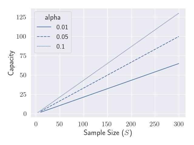
Figure 4: Capacity of an observational study with matched pairs
Figure 4 shows how the capacity increases with the number of pairs for three commonly used significance thresholds. Despite the complicated formula in Equation (\ref{eqn:capacity}), the relationship is fairly linear.
14 Two-Sided Tests
(Rosenbaum 1987) focuses on one-sided tests, but I prefer two-sided tests. A two-sided test may be constructed by doubling the lesser of the p-values for two one-sided tests.
Re-write \( p^u(\gamma) \) as \( p_{>}^u(\gamma) \) to emphasize it is one-sided, with larger values of the test statistic indicating stronger evidence against the null hypothesis. The other one-sided test considers smaller values as stronger evidence. For example, in the test of no effect, when using the mean treatment-minus-control test statistic, a large, negative value would be evidence the treatment is worse than control. If we observed \( W, \) the p-value we would calculate is
\begin{align*} p_< &= \mathrm{Pr}\{ t(d, V) \leq T_\textrm{obs} \, | \, W = w \} \\ &= 1 - \mathrm{Pr}\{ t(d, V) > T_\textrm{obs} \, | \, W = w \} \\ &= 1 - E[ I\{t(d, V) > T_\textrm{obs}\} \, | \, W = w ] \end{align*}
Since \( I\{ t(d, V) > T_\textrm{obs} \} \) is increasing in \( V, \) the expectation is increasing in \( w \) (with respect to \( \preceq_d \)) and the p-value is bounded:
\begin{align*} 1 - \mathrm{Pr}\{ t(d, V) > T_\textrm{obs} \, | \, W = w^u \} &\leq p_< \leq 1 - \mathrm{Pr}\{ t(d, V) > T_\textrm{obs} \, | \, W = w^\ell \} \\ \mathrm{Pr}\{ t(d, V) \leq T_\textrm{obs} \, | \, W = w^u \} &\leq p_< \leq \mathrm{Pr}\{ t(d, V) \leq T_\textrm{obs} \, | \, W = w^\ell \}. \end{align*}
Note the extreme configurations of \( w, \) \( w^\ell \) and \( w^u,\) have switched places compared to (\ref{eqn:p_value_bound}). Thus, \( p_<^u(\gamma) \) is based on \( w^\ell \) while \( p_>^u(\gamma) \) is based on \( w^u. \)
The two-sided p-value we would calculate if we observed \( W \) is \( p_{<>} := 2 \cdot \min\{ p_<, p_>\}. \) The largest \( p_< \) can be is if \( w = w^\ell; \) the largest \( p_> \) can be is if \( w = w^u, \) but these cannot both be true (unless \(\gamma = 0\)). (Rosenbaum 2015, sec. 2.2) mentions this point and suggests calculating
\begin{equation}\label{eqn:p_value_two_sided} p_{<>}^u(\gamma) := 2 \cdot \min\{ p_<^u(\gamma), p_>^u(\gamma)\} \end{equation}
and just accepting that the result will be conservative.
15 Summary
Observational studies involve more uncertainty than randomized experiments because of the possibility of unobserved confounding factors correlated with both treatment and outcome. The first step to managing uncertainty is to quantify is. Paul Rosenbaum has developed an approach to quantifying the uncertainty associated with unobserved confounding called sensitivity analysis.
Unobserved confounding is not about variance, it is about bias. Variance, the primary source of uncertainty in an experiment, can be reduced with larger sample sizes, but bias cannot. As a result, larger sample sizes do not materially affect the sensitivity of an observational study.
Any observational study is invalidated by sufficiently strong unobserved confounding. Every claim from an observational study is a claim, often implicit, about the degree of unobserved confounding. A sensitivity analysis makes the implicit, explicit, by reporting the degree of confounding, \( \Gamma^\star, \) that would invalidate a study’s conclusions.
A p-value facilitates a discussion about the strength of evidence in a randomized experiment. In an observational study, the sensitivity, \( \Gamma^\star, \) plays a similar role. Two experiments with the same p-value offer the same strength-of-evidence. Two observational studies with the same sensitivity do not necessarily offer the same strength-of-evidence. Domain expertise on the treatment selection mechanism must also be applied to assess the plausibility of large hidden biases.